COMPSCI/MATH 290: Spring 2016

• General
• Syllabus
• Assignments
• Final Project
• Raffle

Group Assignment 3: Laplacian Meshes (100 Points)

By Chris Tralie

Click here to see art contest results!

• Overview
  • Deadlines / Points
  • Code Layout/Hints
• Laplacian Mesh Editing
  • Basic Laplacian Mesh Editing (20 Points)
  • Cotangent Weights (20 Points)
  • Smooth Function Interpolation / Mesh Coloring (10 Points)
  • Mesh Sharpening / Smoothing (10 Points)
  • Minimal Surfaces (10 Points)
• Spectral Representations / Heat Flow
  • Laplacian Spectrum (10 Points)
  • Lowpass Geometry Filtering (10 Points)
  • Heat Flow (15 Points)
  • Heat Kernel Signature (10 Points)
• Parameterization / Texturing
  • Mesh Flattening (20 Points)
  • Texture Mapping (10 Points)
• Art Contest
  • Art Contest Submission (5 - 20 Points)

Overview

For the grand finale of the course, students will use Python/Numpy to implement the Laplacian mesh representation, which is a differential operator on the surface of the mesh which approximates the Laplacian of functions on the surface of the mesh. The Laplacian is something like the second derivative along the surface of a function at every point of the mesh, as discussed in class. This representation can be used for a diverse array of tasks in nonrigid geometry processing, such as nonrigid shape editing ("Laplacian mesh editing"), surface function interpolation, compression/denoising, and texture mapping ("uv unwrapping"), to name a few. Students will have an opportunity to implement all of the above operations in this assignment, and this should lead to a rich art contest.

• This assignment was inspired by COS 526 Advanced Computer Graphics: Assignment 2, Fall 2010. Click here to see my writeup for that assignment when I was an undergraduate. I went into a lot of detail, so it will likely help you with your development.

Deadlines / Points

As usual, groups of 1-2 have to earn 100 points, and groups of 3 have to earn 120 points. There will be an intermediate deadline at 11:59PM on Monday 4/18, which is to finish Laplacian Mesh Editing and Cotangent Weights. There will be a 15 point penalty for missing this deadline. The final deadline for the assignment will be on Wednesday 4/27 at 11:59PM.

Code Layout / Hints

Click here to download the code for this assignment

You will be filling in code in the file LaplacianMesh.py, and you will be testing it with a GUI in a file named LapGUI.py. This code runs on a library I made for dealing with meshes in Python called S3DGLPy (the same library that was used to load and sample meshes for the point cloud classification assignment). All of the code you write will be operating on a Python object of type PolyMesh. For this assignment, here's what you need to be aware of:

• All of the vertices are stored in an array mesh.vertices. Each vertex has a field vertex.ID which stores its position in the list. So for instance, mesh.vertices[10].ID is 10
  
  
• Each vertex has a function vertex.getVertexNeighbors() which returns a Python array of the 1-ring neighbors of this vertex, not necessarily in any order
  
  
• The geometry for all of the vertices is stored in an N x 3 numpy array mesh.VPos, which is parallel to the array mesh.vertices. This is the array that you should multiply on the left by the laplacian matrix to get the delta coordinates, and it's also the array you should update after you solve the least squares Laplacian mesh system. Note that points are each along rows now instead of columns in the ordinary convention
  
  
• If two vertices share a neighbor, then passing the corresponding two vertex objects to the function getEdgeInCommon(v1, v2) returns a MeshEdge object representing their edge, or None if they don't share an edge.
  
  
• Each MeshEdge object has two fields f1 and f2 representing the faces on either edge of that edge. Each face is an object of type MeshFace. If the edge is along the boundary, then one or the other will be None. To check to see if f1 is None, for example, the syntax in Python is

  
  if edge.f1:
      print "f1 is not null"
  if not edge.f1:
      print "f1 is null"
  
  

• Each MeshFace object has a function face.getVertices() which returns the vertex objects of that face, not necessarily in any particular order
  
  
• You can check to see if two objects are equal in python with ==
  
  
• When multiplying an ordinary matrix by a sparse matrix, the return type is numpy.matrix instead of numpy.array for some reason. So be sure to case the results as a numpy.array, which is what the rest of the code is expecting. For instance, if you have the Laplacian matrix in a sparse matrix L, then a multiplication by the vertices should be written as

  delta = np.array(L.dot(mesh.VPos))
  

Laplacian Mesh Editing

Note: These laplacian matrices are known to be extremely ill-conditioned, so be sure to fix multiple anchor points where you don't want the surface to move

Basic Laplacian Mesh Editing (20 Points)

• Fill in the functions getLaplacianMatrixUmbrella(mesh, anchorsIdx) and solveLaplacianMesh(mesh, anchors, anchorsIdx)

Set up the Laplacian matrix using umbrella weights and anchors as discussed in class, and solve the system in the least squares sense. You can assume that all anchors have a weight of 1. First, show that you can reconstruct the mesh by fixing one anchor, and then show that the system gives rise to stretching when you fix multiple anchors. To test this, go to the MeshLaplacian menu and click "Select Vertices." Hold SHIFT+Click to select an anchor point, and then hold CTRL + Click to drag that anchor somewhere else. The endpoint of the anchor you are currently selecting is drawn in red, and the endpoint of previously selected anchors is drwan in blue. The image below shows an example:



Then, when you are done, click MeshLaplacian->Solve With Constraints

Cotangent Weights (20 Points)

• Fill in the function getLaplacianMatrixCotangent(mesh, anchorsIdx)

Fill in the laplacian matrix with cotangent weights. That is, fill in the matrix so that \[ L_{ij} = -\frac{1}{2} (\cot(\beta_{ij}) + \cot(\alpha_{ij})) \] and \[ L_{ii} = -\sum_{j = 1, j \neq i}^N L_{ij} \] as shown in the figure below:



You can assume that this is a triangle mesh so that there is exactly one vertex across a face from an edge. Then, change your solveLaplacianMesh() function so that it uses cotangent weights instead of umbrella weights, and highlight the difference on at least one mesh in your README.

Smooth Function Interpolation / Mesh Coloring (10 Points)

• Fill in the function smoothColors(mesh, colors, colorsIdx)

Given a function on the surface of a mesh specified at a few indices, you can do smooth blending of that function across the surface by specifying the function values as anchors in the Laplacian system, and setting the delta coordinates to be zero everywhere. Setting them to zero is like saying the function should minimize the second derivative everywhere, hence the smoothness of the interpolation. You can use this to "color" the entire mesh with very few clicks. In the code, an array called colors is passed along with the RGB values at the indices colorsIdx, and you need to fill in the rest of the colors by doing this function smoothing/completion for each color channel. Below shows an example: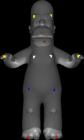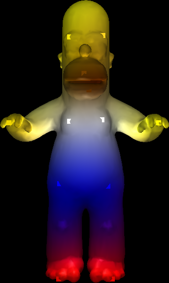

You select the colors in the GUI by going to the menu MeshColoring->Select Color Vertices. Hold down SHIFT + Left Click to select vertices you want to color, just as you did for the Laplacian mesh editor. And then choose their color by holding down CTRL + Left click and clicking on a color in the lower left in the color chooser that's popped up: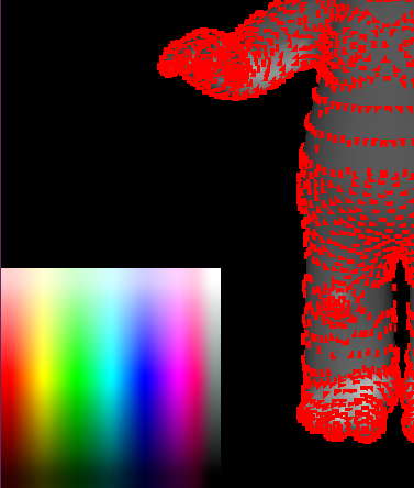



when you've chosen the colors you want, click MeshColoring->Interpolate Colors to test your code

Mesh Sharpening / Smoothing (10 Points)

• Fill in the functions doLaplacianSmooth(mesh) and doLaplacianSharpen(mesh). You can test these by clicking MeshLaplacian->Laplacian Smooth/Sharpen (no anchors needed)

You can use your Laplacian matrix to make simple, efficient surface sharpening and smoothing procedures, which can be shown to work like high and lowpass filters, respectively, by examining their effect on the mesh spectrum. Let L be the square laplacian matrix, and let L_N be the laplacian matrix with each row divided by the sum of the weights of that vertex (so e.g. for umbrella each row should be divided by the degree), so that the diagonal part is all 1s. For the umbrella weights, for example, this normalization gives the vector from the centroid of the neighboring vertices to the vertex. Then to smooth the mesh, apply \[ V' = V - L_N V \] and to sharpen the mesh, apply \[ V' = V + L_N V \]

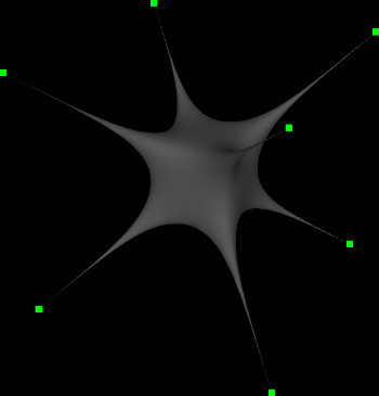
Minimal Surfaces (10 Points)

• Fill in the function makeMinimalSurface(mesh, anchors, anchorsIdx). You can test this by placing anchors and clicking MeshLaplacian->Minimal Surface

A minimal surface is a surface which has a mean curvature of zero, and which equivalently minimizes local surface area. To simulate one, use your original Laplacian matrix (either umbrella or cotangent weights for the purposes of this assignment), but set all delta coordinates to zero. Then, add anchors at particular positions to "anchor" this minimal surface in space with constraints, and apply the least squares laplacian mesh editing. You can think of the anchors as positions along a wire, and the surface as a soap bubble that forms inside of the wires. Click here to see some crazy examples.

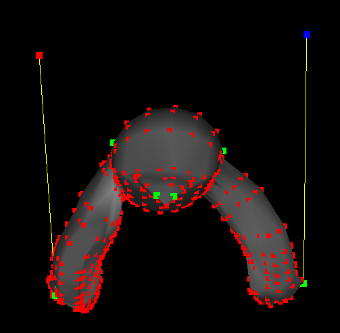
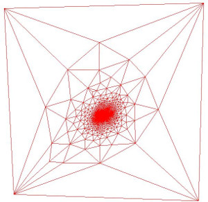
NOTE: For this task, it will work better if instead of having anchors at the bottom, you overwrite the corresponding rows of the upper square laplacian matrix with the anchor rows, and you should do this. So for instance, if you want to anchor a point at index 100 with the position (a, b, c), then row 100 of L should contain all zeros except for a 1 at column 100, and row 100 of the "delta coordinates" should be (a, b, c). The rows corresponding to non-anchor vertices should still be as before, representing the Laplacian at that vertex. Below is an example of the result I got when anchoring the 8 corners of the high resolution cube mesh that way:

Spectral Representations / Heat Flow

Laplacian Spectrum (10 Points)

• Fill in the function getLaplacianSpectrum(mesh, K)

As explained in class, the eigenvectors of the Laplacian matrix are analagous to a Fourier modes of functions along the surface of the mesh. To view the different "modes" of the surface, write code which computes them. To test your code, click MeshLaplacian->GetSpectrum. This code will save SPECTRUM_K modes to a series of .off files "spectrumX.off", where X ranges from 0 to SPECTRUM_K-1. SPECTRUM_K is a constant which is defined at the top of the GUI (default 20), which you can change. You can view the different modes by loading them into the GUI or by looking at them in meshlab

In your readme, explain what you're seeing as you transition from eigenvectors which have small eigenvalues to those which have larger ones.

Lowpass Geometry Filtering (10 Points)

• Fill in the function doLowpassFiltering(mesh, K)

As shown in class, you can do something analagous to a lowpass Fourier filtering by projecting functions onto the lower eigenvectors of the Laplacian matrix of a surface. Let UK be a matrix with the first K eigenvectors in the columns of the matrix, and let V be a matrix with the x coordinates of all of the vertices along the first column, the y coordinates along the second column, and the z coordinates along the third column. Then you can project the coordinates of the geometry onto them with \[ V' = U_K U_K^T V \] Show that you can denoise homernoise.off with this technique. Also show a screenshot on at least one other mesh (lowpassing with very few frequencies looks quite interesting, as shown in class). You can vary the number of eigenvectors you choose by editing the variable LOWPASS_K at the top of the GUI file. Its default value is 20, which is quite low (it takes up to 500 for homer to start looking reasonable, for example, as shown in class)

Heat Flow (15 Points)

• Fill in the function getHeat(mesh, eigvalues, eigvectors, t, initialVertices, heatValue = 100.0)

As shown in class, given an initial heat distribution f₀ over a surface, the solution to the heat equation is

\[ f(t) = \sum_k (f_0^T \phi_k) e^{-\lambda_k t} \phi_k \]

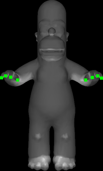
where \phi_k is the k^th eigenvector and \lambda_k is the associated eigenvalue of the laplacian matrix. Given an initial set of point locations "initialVertices," apply "heatValue" amount of heat to them at the beginning of time, and return the amount of heat on all the vertices at time t according to the above equation.

To test this, click on MeshLaplacian->Do Heat Flow Simulation. This will output a bunch of files called heatX.png, where X ranges from 0 to 89 (so you can use this to make a 90 frame vide). To change the number of eigenvectors/eigenvalues used in the computation, feel free to change the variable HEAT_K at the top of the GUI. The more you use, the better the approximation will be for the initial heat distribution (though it won't matter so much after the first few frames since heat dissipates exponentially quickly). Below is an example of selecting the initial conditions as heat on the tips of Homer's 8 fingers

Selecting Initial Heat Vertices	Heat Flow Animation

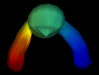
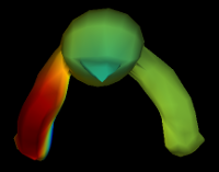
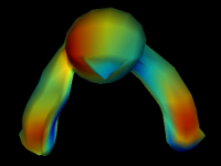
Heat Kernel Signature (10 Points)

• Fill in the function getHKS(mesh, K, t)

As shown in class and described in this paper, a multiscale descriptor of curvature can be computed by looking at how much heat stays at each vertex after a certain amount of time has elapsed, with the following equation:

\[ h_t[i] = \sum_k e^{-\lambda_k t} \phi_k[i]^2 \]

The larger the t, the more the curvature estimate is "regularized" (smoothed out). You can change the variables HKS_K and HKS_T, to change the number of eigenvectors used in the estimate and the time, respectively. Below shows a screenshot of two different times used on the homer mesh

t = 20	t = 500

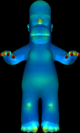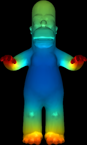Notice how for a smaller t, the curvature on the original fingers is resolvable, whiel in the smoothed version the whole hand contributes to one large curved region all merged together.

Parameterization / Texturing

Mesh Flattening (20 Points)

• Fill in the function doFlattening(mesh, quadIdxs)

You can use Laplacian mesh editing to parameterize a surface with two coordinates. In other words, you can flatten the surface to the plane. To do this, use the Laplacian mesh anchor selector to select four vertices that go in counter-clockwise order around two triangles which share an edge, as shown in the picture below:



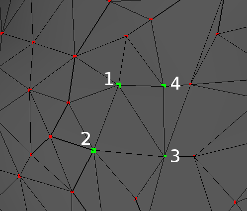
Then, build your laplacian matrix, ignoring the edge that connects the two triangles (effectively removing the two triangle faces from the mesh). Then, set all of the delta coordinates to zero, but put anchors of the four points at (0, 0, 0), (0, 1, 0), (1, 1, 0), and (1, 0, 0). You will want to overwrite rows in the upper square matrix instead of putting the anchors at the bottom, as you did in the minimal surfaces task, and you will also want to use umbrella weights instead of cotangent weights as explained in my undergraduate writeup. When you do all of this and solve the system, the points will try to be the average of their neighbors, and this will have the effect of flattening everything inside of the unit square in the XY plane. Below shows two views of doing this on the homer mesh:



You can test your code out by clicking MeshLaplacian->Do Flattening

Texture Mapping (10 Points)

• Fill in the function getTexCoords(mesh, quadIdxs)

Now that you have a way to flatten the mesh to the plane, you can wrap a texture around it by taking the x coordinate of each point to be the length along the image you want to wrap around and the y coordinate to be the height along the image. This is called UV mapping. Return an N x 2 matrix with the u coordinates of each point along the first column and the v coordinates of each point along the second column. When you test your code by clicking MeshLaplacian->Compute UV Coordinates, the GUI will automatically render a texture on your mesh using the UV coordinates you have. The texture will be whatever you put in the image texture.png (by default, a checkerboard).

Art Contest

Art Contest Submission (5 - 20 Points)

You know the drill by now. 5 points for a submission, 20 points for the winner. The winner's points may be applied towards extra credit, while everyone else's scores are capped at 100%.

Have fun!!